Academic project · University of Aberdeen · September 2026

ECG Classification & Model Evaluation

Comparing classical classifiers with recurrent neural networks on a binary ECG classification task, with attention to baselines, class-level errors, and the value of added model complexity.

Model evaluation

Sequence modelling

Baseline comparison

Error analysis

Models compared: 5
Held-out test samples: 180
Measurements per ECG: 140

The problem

The task is to assign a binary label to an ECG sample containing 140 measurements. I compared KNN and Gaussian Naive Bayes with LSTM, bidirectional LSTM, and GRU networks to investigate whether a recurrent representation improved on classical baselines for the provided dataset.

My contribution

Prepared the course-provided data for static classifiers and reshaped ECG samples to 140-step, single-feature sequences for recurrent models.
Implemented and compared two classical classifiers and three recurrent architectures, with validation-loss early stopping for the neural networks.
Examined accuracy, class-level precision, recall, F1-score, AUROC, confusion matrices, and training histories to compare the approaches.

Approach

Preserve the provided splits
The recurrent experiments use 1,081 training, 541 validation, and 180 test samples. The classical classifiers use the provided training and test partitions.
Establish classical baselines
KNN uses three neighbours and Euclidean distance. Gaussian Naive Bayes uses its default configuration. Both receive a 140-feature vector for each sample.
Train recurrent models
LSTM, bidirectional LSTM, and GRU use stacked recurrent layers, dropout, and a sigmoid output. Training uses Adam, binary cross-entropy, and restoration of the best validation-loss weights.
Compare errors and complexity
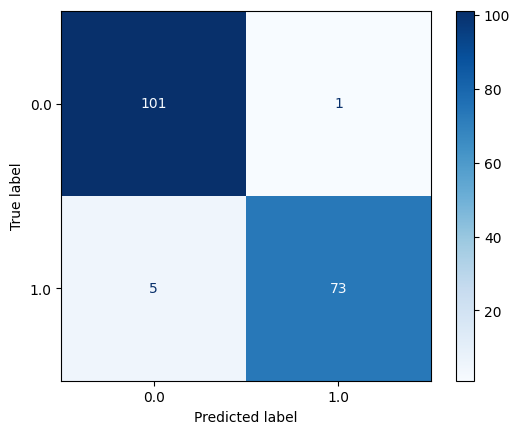
Evaluate all five models on the held-out test partition. Inspect class-1 precision and recall alongside aggregate accuracy, ROC curves, and convergence behaviour.

Results & findings

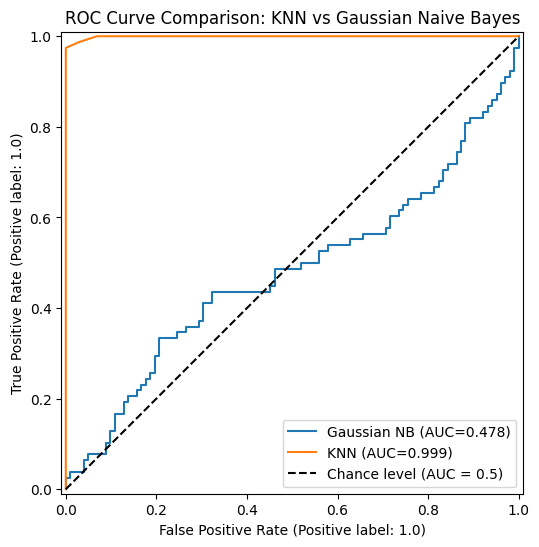
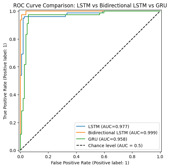
KNN had the highest rounded test accuracy, while the bidirectional LSTM was the strongest recurrent model on that metric. Both recorded an AUROC of 0.999. The additional neural-network complexity did not improve test accuracy over KNN in this experiment.

ECG Classification & Model Evaluation: comparison results
Model	Accuracy	Precision¹	Recall¹	F1¹	AUROC
KNN (k = 3)	0.98	0.96	0.99	0.97	0.999
Gaussian Naive Bayes	0.53	0.45	0.44	0.44	0.478
LSTM	0.96	0.97	0.94	0.95	0.977
Bidirectional LSTM	0.97	0.99	0.94	0.96	0.999
GRU	0.96	0.93	0.97	0.95	0.958

¹ Precision, recall, and F1 refer to class 1. Scores are rounded. Test set: 180 samples.

KNN and bidirectional LSTM made different class-1 trade-offs: KNN recorded recall of 0.99 and precision of 0.96; bidirectional LSTM recorded recall of 0.94 and precision of 0.99.
Gaussian Naive Bayes recorded an accuracy of 0.53 and AUROC of 0.478. Its results underline the importance of checking model assumptions and retaining a useful baseline.
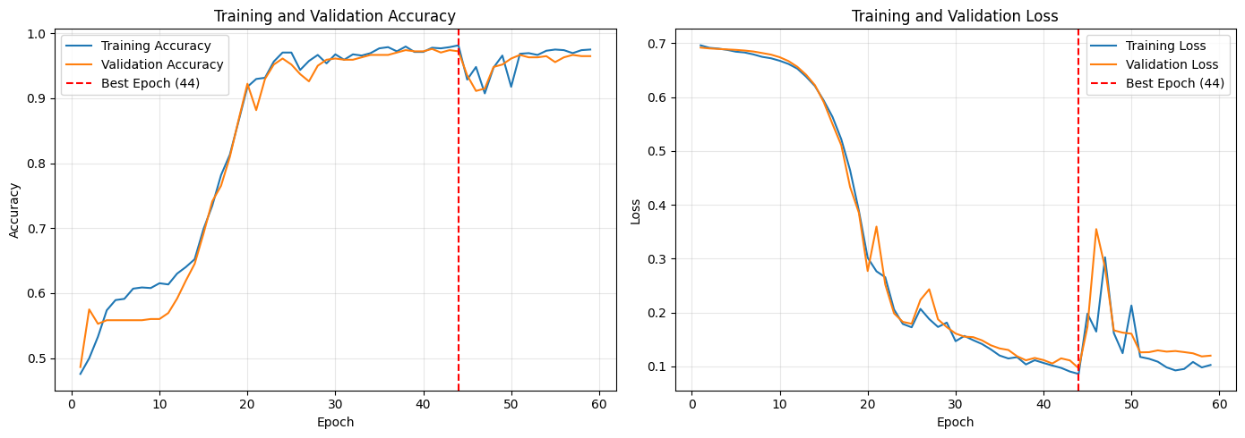
The bidirectional LSTM reached its best validation-loss epoch at 44 in the training history. Early stopping restored those weights after subsequent validation loss stopped improving.

Download results CSV

Experiments & analysis

Select a figure to view it at full size.

Saved ROC curves comparing KNN and Gaussian Naive Bayes on the ECG test set, with AUROC of 0.999 and 0.478 respectively. — ROC comparison of the classical baselines.

Saved ROC curves for LSTM, bidirectional LSTM, and GRU, with AUROC values of 0.977, 0.999, and 0.958 respectively. — ROC comparison of the recurrent models.

Bidirectional LSTM confusion matrix: 101 class-0 samples and 73 class-1 samples classified correctly, with one class-0 and five class-1 errors. — Bidirectional LSTM: the confusion matrix makes the class-level error trade-off visible.

Bidirectional LSTM training and validation accuracy and loss by epoch, with the best validation-loss epoch marked at 44. — Bidirectional LSTM training history. The best validation-loss epoch is marked by the red dashed line.

Inspect the bidirectional LSTM architecture

The model uses two bidirectional recurrent layers, dropout, and a sigmoid output for binary classification.

Python / Keras · Source excerpt

bidirectional_lstm_model = Sequential([
    Input(shape=(140, 1)),
    Bidirectional(LSTM(64, activation='tanh', return_sequences=True)),
    Dropout(0.2),
    Bidirectional(LSTM(32, activation='tanh')),
    Dropout(0.2),
    Dense(16, activation='relu'),
    Dense(1, activation='sigmoid')
])
bidirectional_lstm_model.compile(
    optimizer=keras.optimizers.Adam(learning_rate=0.0001),
    loss=keras.losses.BinaryCrossentropy(),
    metrics=['accuracy']
)

Limitations & what I learned

The held-out test set contains 180 samples. A small number of changed predictions can move the reported scores, so these results have limited precision.
The assessment compares one fixed configuration per model. Repeated seeds, broader hyperparameter tuning, and external datasets are needed to assess how stable the ranking is.
The experiment uses a course-provided dataset and is an academic classification study. It does not establish clinical validity or performance in deployment.

Where I would take this next

Compare repeated runs and validation-selected hyperparameters, and report variation alongside average performance.
Measure inference latency and memory use so model selection can account for deployment constraints as well as predictive scores.

The problem

My contribution

Approach

Preserve the provided splits

Establish classical baselines

Train recurrent models

Compare errors and complexity

Results & findings

Experiments & analysis

Limitations & what I learned

Where I would take this next